Cách dùng keras và tensorflow trong R. So sánh R interface và Python interface cho keras.

Last updated on Sep 1, 2020 5 min read Python, R

Nội dung của bài bao gồm:

1. Cài đặt môi trường làm việc để kết hợp R và Python.

2. So sánh R interface và Python interface cho keras với bài toán MNIST nổi tiếng.

1 Cài đặt

1.1 Cài đặt keras và tensorflow trong R

Để cài đặt Keras và Tensorflow trong R các bạn dùng các lệnh sau:

install.packages("keras")
install.packages(“tensorflow”)
library(keras)
install_keras()

1.2 Cài đặt keras và tensorflow trong Python (sử dụng anaconda)

Để làm việc về khoa học dữ liệu với ngôn ngữ Python, một cách đơn giản nhất là tải về và cài đặt Anaconda - nền tảng (platform) mã nguồn mở về khoa học dữ liệu thông dụng nhất hiện nay hỗ trợ làm việc với Python và R. Nếu chưa biết cách sử dụng R trong Anaconda thì các bạn có thể đọc bài hướng dẫn trước tại đây. Download và cài đặt Anaconda tại đây

Lưu ý: trong khi cài các đặt bạn nhớ là tích vào mục Add Anaconda to my PATH environment variable.

Sau khi đã cài xong Anaconda, các bạn vào Anaconda Prompt để tạo một môi trường mới chứa các thư viện cần thiết như sau:

conda create -n r-env python=3.7 scikit-learn pandas numpy matplotlib keras tensorflow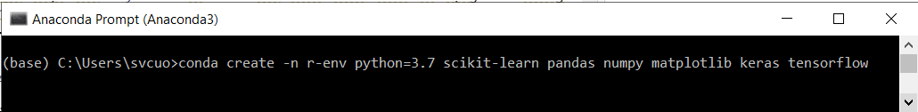

Câu lệnh trên có nghĩa là:

Khởi tạo môi trường anaconda mới với tên r-env
Cài python phiên bản 3.7 với các thư viện scikit-learn, pandas, numpy, matplotlib, keras và tensorflow cho môi trường này

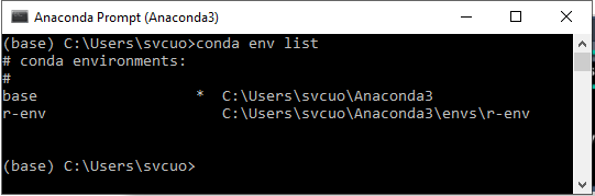
Kiểm tra xem môi trường r-env đã được tạo trong Anaconda chưa bằng lệnh conda env list:

1.3 Thiết lập môi trường làm việc để sử dụng kết hợp R và Python trong R

Để sử dụng Python trong R chúng ta sử dụng gói reticulate. Để biết cách kết hợp R và Python trong R các bạn có thể đọc bài trước tại đây.

Nạp thư viện reticulate và sử dụng hàm conda_list() để kiểm tra danh sách môi trường Anaconda:

library(reticulate)
conda_list()

##    name                                               python
## 1 r-env C:\\Users\\svcuo\\Anaconda3\\envs\\r-env\\python.exe

Vậy là đã có môi trường r-env mới khởi tạo. Để chọn môi trường này sử dụng trong R chúng ta sử dụng hàm use_condaenv():

use_condaenv("r-env")

2. So sánh R interface và Python interface cho keras với bài toán MNIST nổi tiếng

Chú ý: do sử dụng kết hợp R và Python trong cùng một R Notebook nên tôi sẽ chú thích R với mỗi R code chunk và Python với mỗi Python code chunk.

2.1 Sử dụng R interface cho keras

Nạp tập dữ liệu MNIST từ keras:

# R code
library(keras)
mnist <- dataset_mnist()
train_images <- mnist$train$x
train_labels <- mnist$train$y
test_images <- mnist$test$x
test_labels <- mnist$test$y

Kiểm tra dữ liệu:

# R code
dim(train_images)

## [1] 60000    28    28

dim(train_labels)

## [1] 60000

dim(test_images)

## [1] 10000    28    28

dim(test_labels)

## [1] 10000

Thử hiển thị 5th digit:

# R code
digit <- train_images[5,,]
plot(as.raster(digit, max = 255))

Hướng dẫn thao tác với tensors trong R:

# R code
slice1 <- train_images[10:99,,]
dim(slice1)

## [1] 90 28 28

# R code
slice2 <- train_images[10:99,1:28,1:28]
dim(slice2)

## [1] 90 28 28

slice3 <- train_images[, 15:28, 15:28]
dim(slice3)

## [1] 60000    14    14

Thiết kế cấu trúc network model:

# R code
model <- keras_model_sequential() %>%
  layer_dense(units = 512, activation = "relu", input_shape = c(28 * 28)) %>%
  layer_dense(units = 10, activation = "softmax")

Model Summary :

# R code
summary(model)

## Model: "sequential"
## ________________________________________________________________________________
## Layer (type)                        Output Shape                    Param #     
## ================================================================================
## dense (Dense)                       (None, 512)                     401920      
## ________________________________________________________________________________
## dense_1 (Dense)                     (None, 10)                      5130        
## ================================================================================
## Total params: 407,050
## Trainable params: 407,050
## Non-trainable params: 0
## ________________________________________________________________________________

Bước tiếp theo, compile model với loss function, optimizer và metrics tương ứng:

model %>% compile(
  optimizer = "rmsprop",
  loss = "categorical_crossentropy",
  metrics = c("accuracy"))

Chuẩn bị dữ liệu để huấn luyện mô hình:

train_images <- array_reshape(train_images, c(60000, 28 * 28))
train_images <- train_images / 255
test_images <- array_reshape(test_images, c(10000, 28 * 28))
test_images <- test_images / 255

train_labels <- to_categorical(train_labels)
test_labels <- to_categorical(test_labels)

Huấn luyện mô hình:

model %>% fit(
  train_images, 
  train_labels, 
  epochs = 5, 
  batch_size = 128)

Đánh giá độ chính xác của mô hình:

metrics <- model %>% evaluate(test_images, test_labels)
metrics

## $loss
## [1] 0.06532291
## 
## $accuracy
## [1] 0.9802

Dự đoán với dữ liệu mới:

model %>% predict_classes(test_images[1:10,])

##  [1] 7 2 1 0 4 1 4 9 5 9

2.2 Sử dụng Python interface cho keras trong môi trường R

Nạp tập dữ liệu MNIST từ keras:

# Python
from keras.datasets import mnist

## Using TensorFlow backend.

(train_images, train_labels), (test_images, test_labels) = mnist.load_data()

Kiểm tra dữ liệu:

# Python
train_images.shape

## (60000, 28, 28)

# Python
train_labels.shape

## (60000,)

# Python
test_images.shape

## (10000, 28, 28)

# Python
test_labels.shape

## (10000,)

Thiết kế cấu trúc network model:

# Python
from keras import models
from keras import layers

model = models.Sequential()
model.add(layers.Dense(512, activation='relu', input_shape=(28 * 28,)))
model.add(layers.Dense(10, activation='softmax'))

Compile model với loss function, optimizer và metrics tương ứng:

# Python
model.compile(optimizer='rmsprop',
loss='categorical_crossentropy',
metrics=['accuracy'])

Chuẩn bị dữ liệu để huấn luyện mô hình:

# Python
train_images = train_images.reshape((60000, 28 * 28))
train_images = train_images.astype('float32') / 255
test_images = test_images.reshape((10000, 28 * 28))
test_images = test_images.astype('float32') / 255

# Python
from keras.utils import to_categorical
train_labels = to_categorical(train_labels)
test_labels = to_categorical(test_labels)

Huấn luyện mô hình:

# Python
model.fit(train_images, train_labels, epochs=5, batch_size=128)

Đánh giá độ chính xác của mô hình:

# Python
test_loss, test_acc = model.evaluate(test_images, test_labels)

print('test_acc:', test_acc)

## test_acc: 0.980400025844574

Dự đoán với dữ liệu mới:

# Python
model.predict_classes(test_images[:10,:])

## array([7, 2, 1, 0, 4, 1, 4, 9, 5, 9], dtype=int64)

R Markdown Machine Learning Deep Learning Keras Tensorflow

Cuong Sai

PhD student

My research interests include Industrial AI (Intelligent predictive maintenance), Machine and Deep learning, Time series forecasting, Intelligent machinery fault diagnosis, Prognostics and health management, Error metrics / forecast evaluation.